Enclosure indexes • monitoR

Entropy

This is based on @brereton-2022. First we count the number of observations in each grid. Then we have

$p_i = X_i / N, i=1, \dots, k$

where $p_i$ is the proportion of observation in grid $i$ , $X_i$ is the number of observations in grid $i$ , and finally $N$ is the total number of observations.

The entropy is then $E_i = -\sum^k_{i = 1}p_i\log_{10}(p_i)$

Note that we use Base 10 log, originally entropy is base 2, but the behaviourists seem to use 10,
we define $0\log_{10}(0) = 0$ , and
This lies between 0 and $log_{10}(k)$

If all the observations lie in one grid then we have

$-(0 + 0 + \dots + 1\log_{10}(1) + \dots + 0) = 0$

If the data is evenly spread, then

$p_i = \frac{1}{k}$

So we have

$-\sum^k_{i = 1}\frac{1}{k}\log_{10}\left(\frac{1}{k}\right) = \sum^k_{i = 1}\frac{1}{k}\log_{10}(k) = \log_{10}(k)$

For a empirical p-value for entropy - see ?@sec-entropy-pv.

Modified spread of participation index (SPI)

From @plowman-2003, we have

$SPI = \frac{\sum_{i = 1}^k\mid f^o_i - f^e_i \mid}{2(N - \min_{i = 1, \dots, k}(f^e_{i}))},$

where

$k$ is the number of zones,
$f_i^o$ is the observed frequency in zone $i$ ,
$f_i^e$ is the expected frequency in zone $i$ ,
$N$ is the total number of observations:

$N= \sum^k_{i = 1}f_i^o$

Figure 1: Simulated dataset with even spread

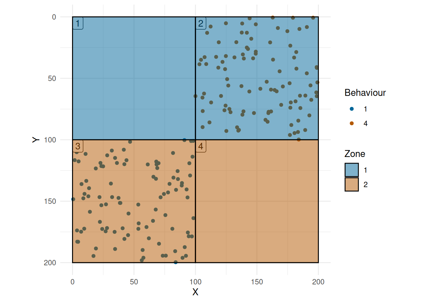
For even spread, we should have a SPI of zero. To test this, consider the simulated data given in Figure 1, in this case, we have four grids, two with 100 points each - Grid 2 and Grid 3. Also we have two zones:

Zone 1: Grid 1 and Grid 2,
Zone 2: Grid 3 and Grid 4.

In this case, we have

$k = 2$ ,
$f^o_1 = f^o_2 = 100$ ,
$N = 200$ , and
$f^e_1 = f^e_2 = 200 / 4 \times 2 = 100$ .

Putting this together gives SPI = 0,

get_zone_object(grid_even, obs) |> calc_spi()
#> [1] 0

Now, we consider the uneven case (Figure 2), in this case, we have the same points, 100 in Grid 3 and 100 in Grid 2, but now all the points appear in Zone 2, and none in Zone 1. So now we have

$k = 2$ ,
$f^o_1 = 200$
$f^o_2 = 0$ ,
$N = 200$ , and
$f^e_1 = f^e_2 = 200 / 4 \times 2 = 100$ .

plot_grid(grid_uneven, obs, grid_col = TRUE, zone_fill = TRUE)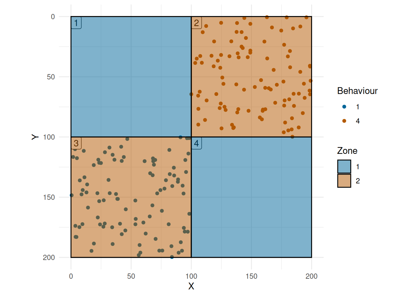

This gives the largest possible modified SPI of

get_zone_object(grid_uneven, obs) |> calc_spi()
#> [1] 1

Electivity Index

From @brereton-2022, we have

$E = \frac{W_i - 1/n}{W_i + 1/n},$ where $W_i = \frac{r_i/p_i}{\sum_{i=1}^nr_i/p_i},$ where $n$ is the number of zones, $r_i$ is the proportion number of observations in zone $i$ , and $p_i$ is the expected proportion of observations based on equal grid use.

Consider the case of even spread (Figure 1), this gives a EI of

get_zone_object(grid_even, obs) |>
  calc_ei() |>
  dplyr::select(zone, ei) |>
  gt::gt()

zone	ei
1	0
2	0

so zero for each zone. While in the case of uneven spread (Figure 2), we have an EI of

get_zone_object(grid_uneven, obs) |>
  calc_ei() |>
  dplyr::select(zone, ei) |>
  gt::gt()

zone	ei
1	0.3333333
2	-1.0000000

Note that -1 indicates no use, and the 0.33 indicates sole use. The 0.33 is $(n-1)/(n+1)$ which goes to 1 as $n$ gets large