pacman::p_load(tidyverse, gt, monitoR)
theme_set(theme_bw())
Load data
data(cassowary)
cassowary |> glimpse()
#> Rows: 4,350
#> Columns: 7
#> $ time         <dttm> 2023-09-08 15:02:58, 2023-09-08 15:02:58, 2023-09-08 15:…
#> $ X            <dbl> 285, 322, 282, 322, 283, 277, 279, 267, 273, 316, 277, 36…
#> $ Y            <dbl> 329, 366, 330, 227, 306, 215, 324, 212, 342, 264, 353, 25…
#> $ behaviour    <chr> "Laying Down (Ld)", "Repetitive Behaviour (Rb)", "Laying …
#> $ cassowary    <chr> "Jeffrey", "Martina", "Jeffrey", "Martina", "Jeffrey", "M…
#> $ jeffery_side <chr> "Left", "Left", "Left", "Left", "Left", "Left", "Left", "…
#> $ martina_side <chr> "Right", "Right", "Right", "Right", "Right", "Right", "Ri…
Adding the grid
We add a 4x4 grid - decide to make a bit nicer than the default grid. Note that there are two zones denotes left and right (Figure 1).
grid <- create_grid(
  range(cassowary$X),
  range(cassowary$Y),
  dim = c(4, 4)
)
grid <- grid |>
  mutate(
    left = case_when(
      left == 74 ~ 0,
      left == 195.25 ~ 150,
      left == 316.5 ~ 300,
      left == 437.75 ~ 450,
      TRUE ~ left
    ),
    right = case_when(
      right == 74 ~ 0,
      right == 195.25 ~ 150,
      right == 316.5 ~ 300,
      right == 437.75 ~ 450,
      right == 559 ~ 600,
      TRUE ~ right
    )
  )
grid$zone <- "right"
grid$zone[c(1, 2, 5, 6, 9, 10, 13, 14)] <- "left"
cassowary_grid <- cassowary |> add_grid(grid)
plot_grid(grid, cassowary_grid, zone_fill = TRUE) +
  theme(legend.position = "none")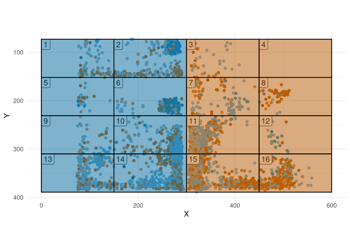
Cassowary side
We have two cassowaries - Martina and Jeffrey. They are let out into on of the sides. We have information about which side they are in.
martina <- cassowary_grid |>
  filter(cassowary == "Martina")
jeffrey <- cassowary_grid |>
  filter(cassowary == "Jeffrey")
jeffrey
#> # A tibble: 2,174 × 9
#>    time                    X     Y behaviour cassowary jeffery_side martina_side
#>    <dttm>              <dbl> <dbl> <chr>     <chr>     <chr>        <chr>
#>  1 2023-09-08 15:02:58   285   329 Laying D… Jeffrey   Left         Right
#>  2 2023-09-08 15:03:58   282   330 Laying D… Jeffrey   Left         Right
#>  3 2023-09-08 15:04:58   283   306 Laying D… Jeffrey   Left         Right
#>  4 2023-09-08 15:05:58   279   324 Laying D… Jeffrey   Left         Right
#>  5 2023-09-08 15:06:58   273   342 Laying D… Jeffrey   Left         Right
#>  6 2023-09-08 15:07:58   277   353 Laying D… Jeffrey   Left         Right
#>  7 2023-09-08 15:08:58   287   352 Laying D… Jeffrey   Left         Right
#>  8 2023-09-08 15:09:58   282   369 Laying D… Jeffrey   Left         Right
#>  9 2023-09-08 15:10:58   284   370 Laying D… Jeffrey   Left         Right
#> 10 2023-09-08 15:11:58   166   217 Locomoti… Jeffrey   Left         Right
#> # ℹ 2,164 more rows
#> # ℹ 2 more variables: grid <dbl>, zone <chr>
Figure 2 gives the positions for Martina and also the side that she is recorded on, while Figure 3 gives the equivalent for Jeffrey.
Note
Need to discuss with EF.
grid |>
  ggplot2::ggplot() +
  ggplot2::geom_rect(
    ggplot2::aes(xmin = left, xmax = right, ymin = bottom, ymax = top),
    col = "black",
    alpha = 0.1,
    fill = NA
  ) +
  ggplot2::geom_point(
    ggplot2::aes(X, Y, col = martina_side),
    data = martina
  ) +
  harrypotter::scale_colour_hp_d("Ravenclaw")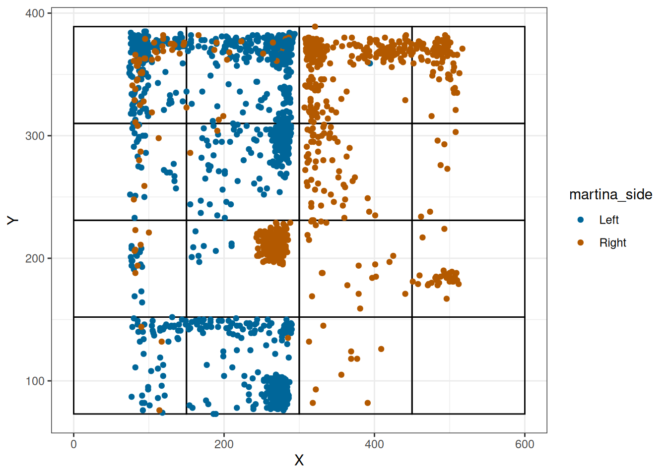
grid |>
  ggplot2::ggplot() +
  ggplot2::geom_rect(
    ggplot2::aes(xmin = left, xmax = right, ymin = bottom, ymax = top),
    col = "black",
    alpha = 0.1,
    fill = NA
  ) +
  ggplot2::geom_point(
    ggplot2::aes(X, Y, col = jeffery_side),
    data = jeffrey
  ) +
  harrypotter::scale_colour_hp_d("Ravenclaw")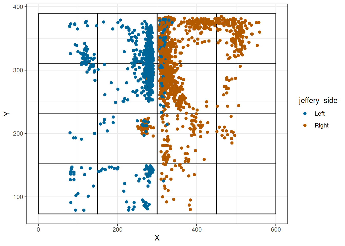
Figure 4 gives the proportion of time that each cassowary is in each grid for the left side.
cassowary_grid |>
  filter(zone == "left") |>
  count(grid, cassowary) |>
  mutate(
    N = sum(n),
    .by = cassowary,
  ) |>
  mutate(
    p = n / N,
    grid = factor(
      grid,
      levels = c(13, 14, 15, 16, 9, 10, 11, 12, 5, 6, 7, 8, 1, 2, 3, 4)
    )
  ) |>
  ggplot(aes(cassowary, p, fill = cassowary)) +
  geom_col() +
  facet_wrap(~grid, ncol = 2) +
  harrypotter::scale_fill_hp_d("Ravenclaw")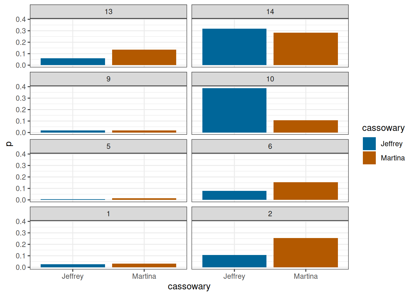
cassowary_grid |>
  filter(zone == "right") |>
  count(grid, cassowary) |>
  mutate(
    N = sum(n),
    .by = cassowary,
  ) |>
  mutate(
    p = n / N,
    grid = factor(
      grid,
      levels = c(13, 14, 15, 16, 9, 10, 11, 12, 5, 6, 7, 8, 1, 2, 3, 4)
    )
  ) |>
  ggplot(aes(cassowary, p, fill = cassowary)) +
  geom_col() +
  facet_wrap(~grid, ncol = 2) +
  harrypotter::scale_fill_hp_d("Ravenclaw")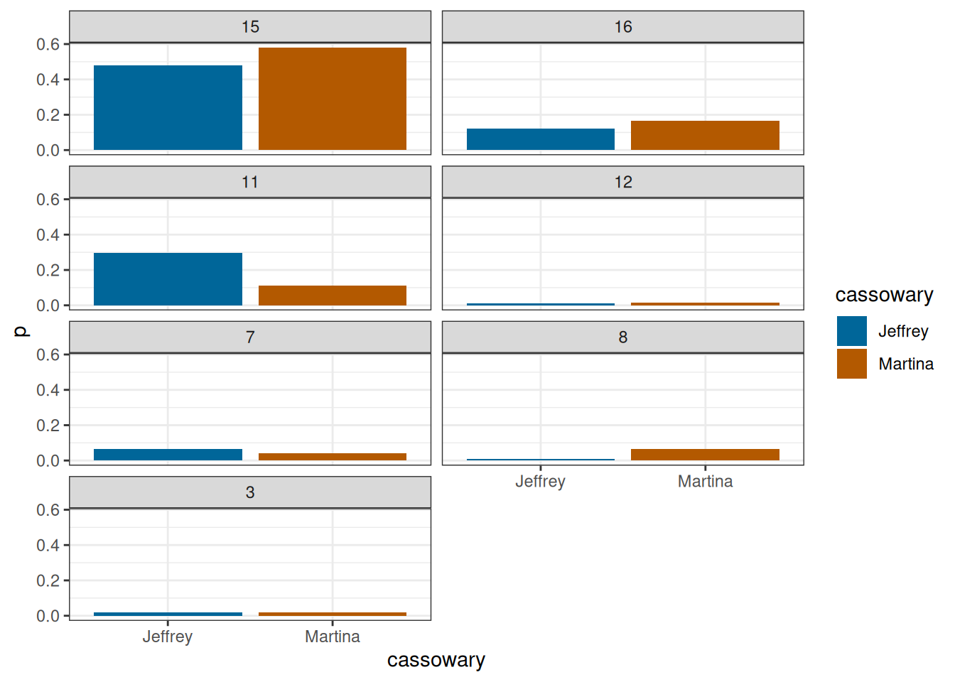
Diversity measures
Entropy
We see that Martina utilises more of the grid than Jeffrey (Table 1)
cassowary_grid |>
  group_by(cassowary) |>
  summarise(entropy = calc_entropy(grid)) |>
  gt() |>
fmt_number(decimals = 4)| cassowary | entropy |
|---|---|
| Jeffrey | 0.8952 |
| Martina | 0.9487 |
Figure 6 gives the entropy for each behaviour for each cassowary.
cassowary_grid |>
  group_by(cassowary, behaviour) |>
  summarise(entropy = calc_entropy(grid)) |>
  filter(entropy > 0) |>
  group_by(behaviour) |>
  mutate(m = max(entropy)) |>
  ungroup() |>
  mutate(
    behaviour = fct_reorder(behaviour, m)
  ) |>
  ggplot(aes(entropy, behaviour, fill = cassowary)) +
  geom_col(position = "dodge") +
  harrypotter::scale_fill_hp_d("Ravenclaw") +
  labs(x = "Entropy", y = NULL)
#> `summarise()` has grouped output by 'cassowary'. You can override using the
#> `.groups` argument.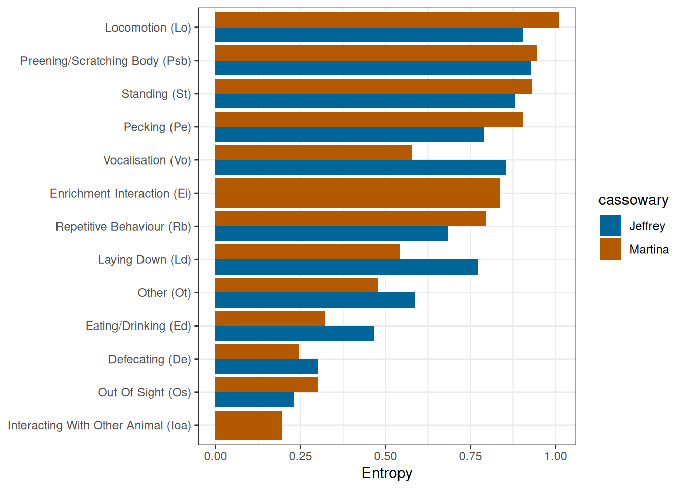
get_zone_object(grid, martina) |> calc_ei()
#> # A tibble: 2 × 8
#>   zone    obs n_grids    ri    pi ratio    wi     ei
#>   <chr> <dbl>   <int> <dbl> <dbl> <dbl> <dbl>  <dbl>
#> 1 left   1684       8 0.774   0.5 1.55  0.774  0.215
#> 2 right   492       8 0.226   0.5 0.452 0.226 -0.377
get_zone_object(grid, jeffrey) |> calc_ei()
#> # A tibble: 2 × 8
#>   zone    obs n_grids    ri    pi ratio    wi     ei
#>   <chr> <dbl>   <int> <dbl> <dbl> <dbl> <dbl>  <dbl>
#> 1 left    805       8 0.370   0.5 0.741 0.370 -0.149
#> 2 right  1369       8 0.630   0.5 1.26  0.630  0.115
get_zone_object(grid, martina) |> calc_spi()
#> [1] 0.5477941
get_zone_object(grid, jeffrey) |> calc_spi()
#> [1] 0.2594296