Analysis of skink dataset • monitoR

library(monitoR)
pacman::p_load(conflicted, tidyverse, gt)
theme_set(theme_bw())

Data

data(skink, package = "monitoR")

skink |> glimpse()
#> Rows: 6,728
#> Columns: 4
#> $ time      <dttm> 2024-03-25 14:34:01, 2024-03-25 14:35:01, 2024-03-25 14:36:…
#> $ X         <dbl> 229, 248, 235, 250, 252, 248, 255, 256, 190, 141, 250, 261, …
#> $ Y         <dbl> 213, 200, 221, 207, 214, 215, 275, 283, 370, 401, 243, 231, …
#> $ behaviour <chr> "Basking", "Basking", "Basking", "Movement", "Basking", "Bas…

Processing

First we add a 4x4 grid

grid <- create_grid(range(skink$X), range(skink$Y), dim = c(4, 4))
skink_grid <- skink |> add_grid(grid)

plot_grid(grid, skink_grid)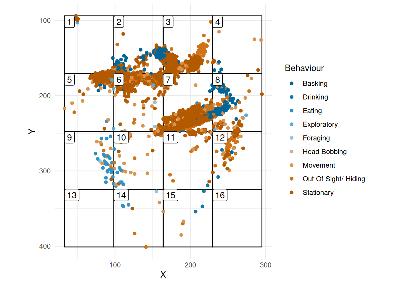

Index measures

Entropy

First we look at the entropy of observation for the data given in Figure 1.

calc_entropy(skink_grid$grid)
#> [1] 0.7944013

Q1: Is it evenly spread? We know that the entopy for evenly spread data over a 4x4 grid using $\log_{10}$ is

$\log_{10}(16)$

log10(16)
#> [1] 1.20412

In our case, we have 0.7944013 which is smaller indicating non-even spread. We may wonder if this is significant?

To test this, we will create a empirical null distribution based on simulating data with equal spread of grids

null_entropy <- monitoR::get_entropy_null(
  skink_grid$grid,
  n_sims = 1000,
  n_grid = 16
)

If we look at the 95% percentiles

quantile(null_entropy, c(0.025, 0.975))
#>     2.5%    97.5% 
#> 1.203245 1.203926

we see that it does not contain the observed value, so the observations are not evenly spread.

Entropy and behaviour

Next, we will calculate the entropy for each behaviour (Figure 2). In this we see a difference in entropy for different behaviours. For example, the most evenly spread is movement, while foraging is the least spread.

skink_grid |>
  summarise(entropy = calc_entropy(grid), .by = behaviour) |>
  mutate(
    behaviour = fct_reorder(behaviour, entropy)
  ) |>
  ggplot(aes(entropy, behaviour, fill = behaviour)) +
  geom_col(show.legend = FALSE) +
  harrypotter::scale_fill_hp_d("Ravenclaw") +
  labs(x = "Entropy", y = NULL)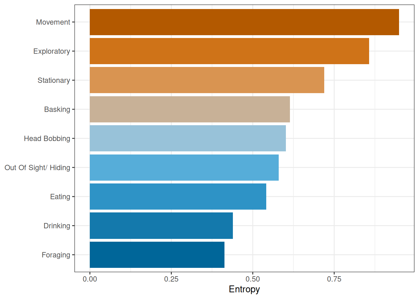

To assess the difference between the entropy for the different behaviours, we will used the squared distance of each entropy from the overall entropy

$ESS = \sum^k_{i = 1} (E_i - E_{\bullet})^2,$

where $E_i$ is the entropy for the $i$ th behaviour, and $E_{\bullet}$ is the entropy for all observations.

For Figure 2, we have

get_ess(skink_grid)
#> [1] 0.4849358

As before, the question is

Is this significant?

To access this, we will use a permutation test, so we will

Permute the grid recorded in the data
Calculate ESS each time

ess_null <- get_ess_null(skink_grid, n_sims = 100)
quantile(ess_null, c(0.025, 0.975))
#>      2.5%     97.5% 
#> 0.1483959 0.8317398

So this time we find that the observed ESS is within the 95% empirical confidence interval and so is not surprising.

Environment effects

So, we will now focus on Basking (Figure 3). We will assume for illustration that there are rocks in Grid 5, 6, 7, 8, 2, and 3.

We want to ask the question of

Is it more likely to bask where there are rocks?

skink_bask <- skink_grid |>
  filter(behaviour == "Basking")

plot_grid(grid, skink_bask)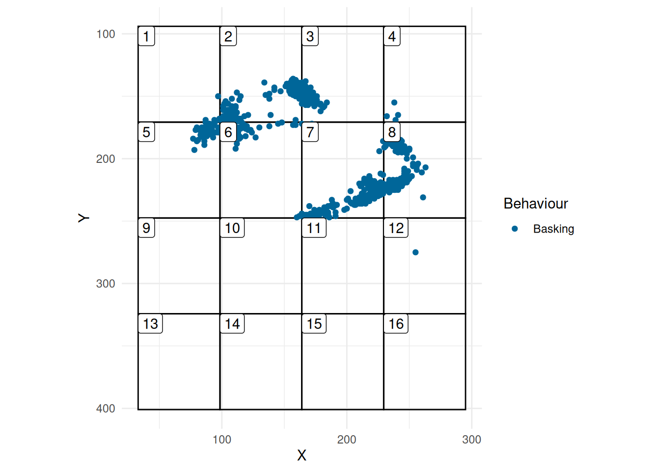

Figure 3: Observations where just basking

Table 1 gives the number of times that the skink is seen basking in each grid. As well, we have given the type of environment.

basking_df <- count_grid_behaviour(grid = grid, skink_bask)
basking_df <- basking_df |>
  mutate(
    environ = "normal"
  )
basking_df$environ[c(2, 3, 5, 6, 7, 8)] <- "rocks"
basking_df |> gt()

Table 1: Count of number of basking events for each grid.

grid	obs	environ
1	5	normal
2	684	rocks
3	126	rocks
4	4	normal
5	36	rocks
6	47	rocks
7	199	rocks
8	166	rocks
9	0	normal
10	0	normal
11	7	normal
12	1	normal
13	0	normal
14	0	normal
15	0	normal
16	0	normal

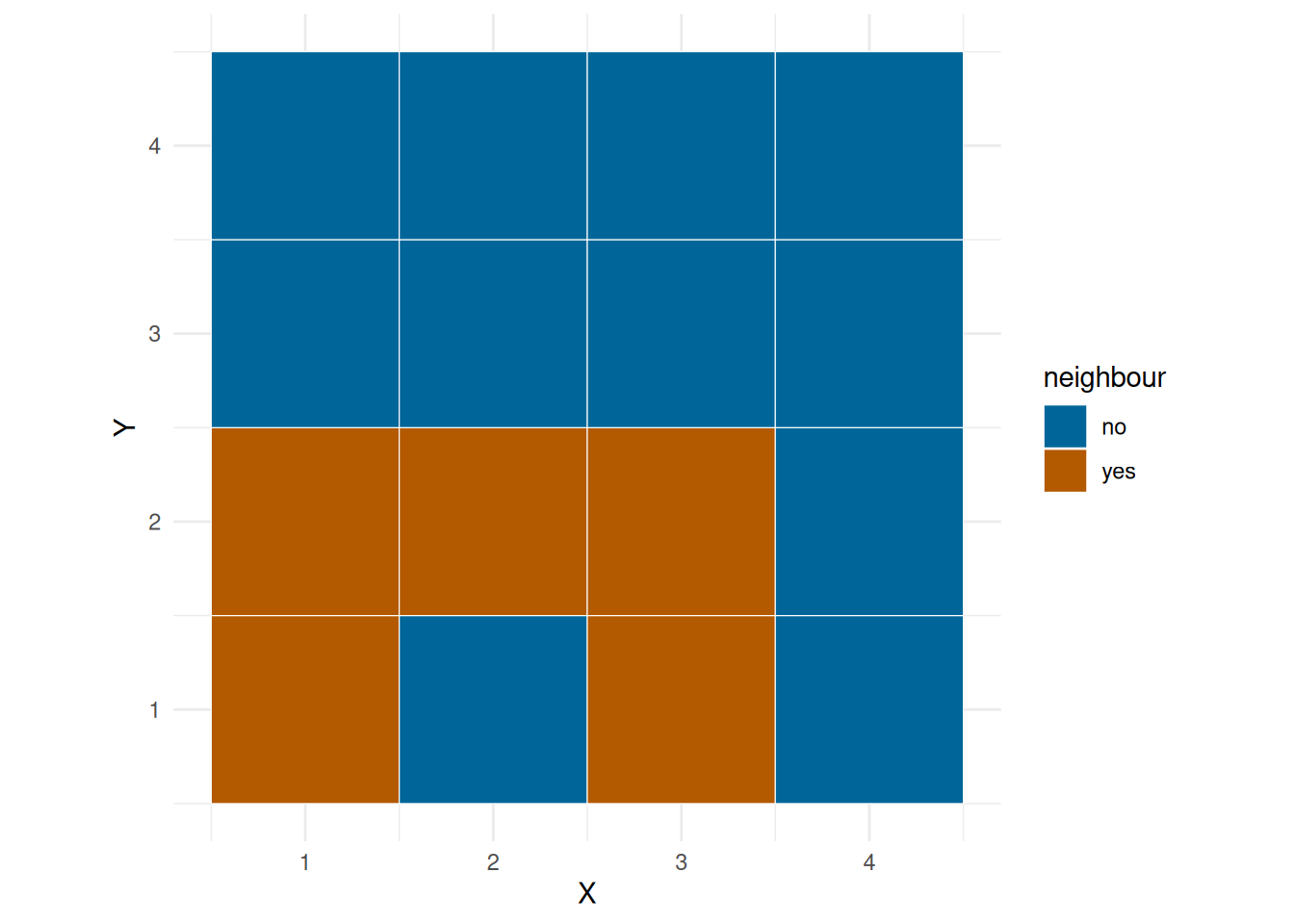
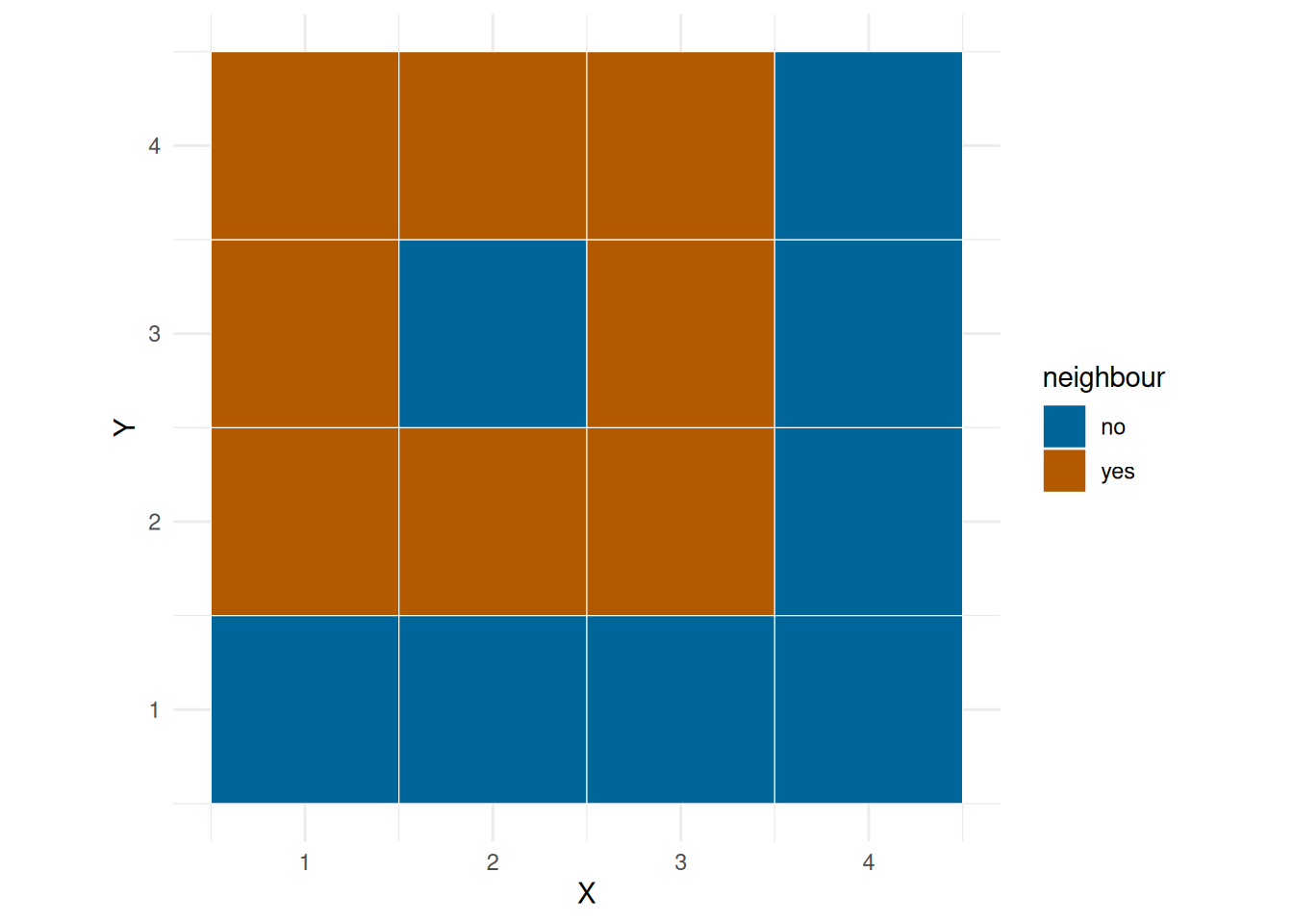
We can fit a linear model of number of observations on environ, but we would also like to take into account the spatial dependency, that is, you will might be more likely to bask in grid next to one another. ?@fig-neigh show the neighbourhood of a corner grid, edge grid and a middle grid.

plot_neigh(grid, 1)
plot_neigh(grid, 2)
plot_neigh(grid, 10)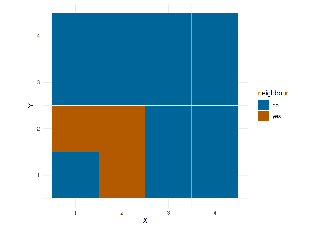

First we add the neigh mean.

M <- get_neigh_mat(grid)
basking_df$neigh <- as.numeric(M %*% basking_df$obs)
basking_df
#> # A tibble: 16 × 4
#>     grid   obs environ  neigh
#>    <dbl> <dbl> <chr>    <dbl>
#>  1     1     5 normal  256.  
#>  2     2   684 rocks    82.6 
#>  3     3   126 rocks   220   
#>  4     4     4 normal  164.  
#>  5     5    36 rocks   147.  
#>  6     6    47 rocks   132.  
#>  7     7   199 rocks   129.  
#>  8     8   166 rocks    67.4 
#>  9     9     0 normal   16.6 
#> 10    10     0 normal   36.1 
#> 11    11     7 normal   51.6 
#> 12    12     1 normal   74.4 
#> 13    13     0 normal    0   
#> 14    14     0 normal    1.4 
#> 15    15     0 normal    1.6 
#> 16    16     0 normal    2.67

And then fit some models

M1 <- lm(obs ~ environ * neigh, data = basking_df)
summary(M1)
#> 
#> Call:
#> lm(formula = obs ~ environ * neigh, data = basking_df)
#> 
#> Residuals:
#>     Min      1Q  Median      3Q     Max 
#> -174.75   -3.78   -0.61   -0.30  375.19 
#> 
#> Coefficients:
#>                    Estimate Std. Error t value Pr(>|t|)  
#> (Intercept)          0.4625    54.1866   0.009   0.9933  
#> environrocks       481.9039   167.0120   2.885   0.0137 *
#> neigh                0.0205     0.5367   0.038   0.9702  
#> environrocks:neigh  -2.1217     1.2582  -1.686   0.1175  
#> ---
#> Signif. codes:  0 '***' 0.001 '**' 0.01 '*' 0.05 '.' 0.1 ' ' 1
#> 
#> Residual standard error: 137.3 on 12 degrees of freedom
#> Multiple R-squared:  0.5002, Adjusted R-squared:  0.3752 
#> F-statistic: 4.003 on 3 and 12 DF,  p-value: 0.03452
M2 <- update(M1, . ~ . - environ:neigh)
summary(M2)
#> 
#> Call:
#> lm(formula = obs ~ environ + neigh, data = basking_df)
#> 
#> Residuals:
#>     Min      1Q  Median      3Q     Max 
#> -167.30  -30.50  -20.25    2.68  457.09 
#> 
#> Coefficients:
#>              Estimate Std. Error t value Pr(>|t|)  
#> (Intercept)   23.7684    55.9865   0.425   0.6781  
#> environrocks 233.3370    83.9025   2.781   0.0156 *
#> neigh         -0.3655     0.5187  -0.705   0.4934  
#> ---
#> Signif. codes:  0 '***' 0.001 '**' 0.01 '*' 0.05 '.' 0.1 ' ' 1
#> 
#> Residual standard error: 146.8 on 13 degrees of freedom
#> Multiple R-squared:  0.3817, Adjusted R-squared:  0.2866 
#> F-statistic: 4.013 on 2 and 13 DF,  p-value: 0.04391
M3 <- update(M2, . ~ . - neigh)
summary(M3)
#> 
#> Call:
#> lm(formula = obs ~ environ, data = basking_df)
#> 
#> Residuals:
#>     Min      1Q  Median      3Q     Max 
#> -173.67  -18.92   -1.70    0.05  474.33 
#> 
#> Coefficients:
#>              Estimate Std. Error t value Pr(>|t|)  
#> (Intercept)      1.70      45.57   0.037   0.9708  
#> environrocks   207.97      74.41   2.795   0.0143 *
#> ---
#> Signif. codes:  0 '***' 0.001 '**' 0.01 '*' 0.05 '.' 0.1 ' ' 1
#> 
#> Residual standard error: 144.1 on 14 degrees of freedom
#> Multiple R-squared:  0.3581, Adjusted R-squared:  0.3123 
#> F-statistic: 7.811 on 1 and 14 DF,  p-value: 0.01433

So it looks like there is no dependency.